LINEAR ALGEBRA NOTES

Notes

“It’s all right there and when I find it there be a hole the size of the everfall that I’ll be able to look through. And on every single level, Rows of doors waiting to be opened.”

I need to figure out how to fluidly intuitively know that relationships between matrices and graphs and category theory and logic and machine learning.

can all graph expressions be represented by a matrix

Are there analogs for graph algorithms that can be done in linear algebra world instead?

I might be able to use adjacency matrices and the graphs for category theory to kind of like recurse use the thing to look back in on itselfですね?

AQSC - A quick steep climb up linear algebra

Notes

ch 7 applications

Adjacency matrix properties

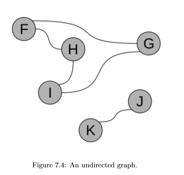
Undirected

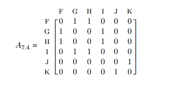
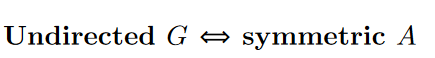If the graph is undirected, its adjacency matrix will be symmetric.

This is, of course, a natural consequence of what “undirected” means. If a graph has no arrowheads, then every time you can go from X to Y, you can also go from Y to X. So if A’s entry at row X and column Y is a 1, then the entry at row Y and column X must also be a 1. And that’s what makes a matrix symmetric.

REMARK: symmetry

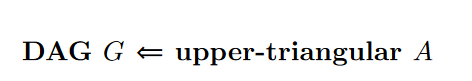
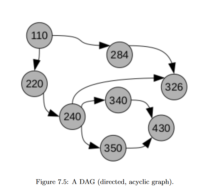
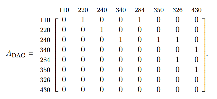
DAG

Disconnected

Disconnected G ⇐ block diagonal A

uppose we have a disconnected graph, like:

This disconnectedness is apparent from the adjacency matrix, because it is get this – block diagonal!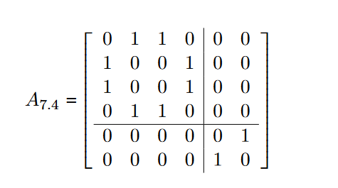

a disconnected graph is separable into isolated subgraphs. (This is a partition, if you remember your set theory from Cool BriskWalk) #### 6.13. THE CENTRAL DOGMA OF SQUARE MATRICES 171

The following things are all true for yellow matrices: • A is a non-singular square matrix. • A has all linearly independent columns (yellow dominoes). • A is “full rank.” (The rank is equal to the dimension of the matrix.) • The kernel of A has only the zero vector in it. • The nullity of A is 0. • A has an inverse matrix, which we can call A−1. • A represents a system of equations which can be solved (and which has exactly one solution.) • A represents a linear transformation that is bijective.

On the flip side, the following are all true for blue matrices: • A is a singular square matrix. • A’s columns are not linearly independent (blue domi- noes). • A is “rank-deficient.” (The rank is less than the dimen- sion of the matrix.) • The kernel of A has more than just the zero vector in it. • The nullity of A is greater than 0. • There is no inverse matrix of A. • A represents a system of equations which either can’t be solved, or which has infinitely many solutions. • A represents a linear transformation that is neither injec- tive nor surjective.

Either all the stuff in the first box is true, or all the stuff in the second box. There is no in between.

Linear operators

The examples provided are some of the common special ( 2 ) linear operators, but there are other notable ones as well. Here’s an expanded list:

1. Identity Operator

] - Leaves vectors unchanged.

2. Zero Operator

] - Maps every vector to the zero vector.

3. Rotation Operator

] - Rotates vectors by an angle ( ). (explination)[here]

4. Scaling Operator

] - Scales vectors by a factor of ( a ).

5. Shear Operator

] - Shears the shape of an object.

6. Reflection Operator

] - Reflects vectors across specified lines or axes.

7. Projection Operator

] - Projects vectors onto specified axes.

These operators cover a broad range of transformations, illustrating the key properties of linearity (additivity and homogeneity) and providing context for understanding linear operators in ( ^2 ).

Rotation Matrix

To understand the rotation operator ( R() ) and how it rotates vectors by an arbitrary angle ( ), let’s start by revisiting some basic concepts and then delve into the specifics of the rotation matrix.

Unit Circle and Basic Trigonometry

The unit circle is a circle with a radius of 1 centered at the origin (0, 0) in the coordinate plane. Any point on the unit circle can be described using the angle ( ) it makes with the positive x-axis. This point has coordinates ( (, ) ).

Rotation Matrix Intuition

The rotation matrix ( R() ) is used to rotate a vector in the plane by an angle ( ). To see why the matrix takes the form it does, let’s consider how it affects a point ( (x, y) ).

Given a point ( (x, y) ), when we rotate it by an angle ( ), the new coordinates ( (x’, y’) ) can be derived from the trigonometric relationships on the unit circle. Here’s a step-by-step breakdown:

1. Original Point Representation:
   • Let’s represent the point ( (x, y) ) in terms of a vector ( = ).
2. Rotated Point Representation:
   • The new coordinates ( (x’, y’) ) after rotation can be found using trigonometric identities: [ x’ = x - y ] [ y’ = x + y ]
3. Matrix Form:
   • We can express these equations in matrix form as: [ = ]
   • This matrix is the rotation matrix ( R() ): [ R() = ]

Example Calculation

Let’s work through a concrete example to see the rotation matrix in action.

) and we want to rotate it by ( = 90^) (or (= ) radians).

1. Rotation Matrix for ( = 90^): [ R() =

   =

   ]

2. Applying the Rotation Matrix: [ ’ = R() =

   =

   ]

   • The vector ( ) has been rotated by ( 90^) to become ( ’ = ).

Summary

• The rotation matrix ( R() ) rotates vectors in the plane by an angle ( ).
• It uses the trigonometric functions cosine and sine to transform the coordinates.
• You can apply ( R() ) to any vector to find its new position after rotation by multiplying the matrix by the vector.

Understanding the rotation matrix involves recognizing how trigonometric functions describe the new coordinates of a point after rotation, leveraging basic concepts from the unit circle and trigonometry.

Minkowski distance

Certainly! Let’s explore the Minkowski distance and its special cases (Manhattan and Euclidean distances), and how you can use different ( p ) values to achieve different distance metrics.

1. Introduction to Minkowski Distance:

The Minkowski distance is a generalized distance metric that defines the distance ( D ) between two points ( (x_1, y_1) ) and ( (x_2, y_2) ) in a 2-dimensional space as:

[ D = ( |x_2 - x_1|^p + |y_2 - y_1|^p )^{1/p} ]

Here, ( p ) is a parameter that determines the type of distance metric:

• Manhattan Distance (p = 1): [ D_{} = |x_2 - x_1| + |y_2 - y_1| ] This measures the sum of the absolute differences in the x and y coordinates, which corresponds to the distance traveled along grid lines (like walking along city blocks).

• Euclidean Distance (p = 2): [ D_{} = ] This is the straight-line distance between the two points in a plane, which is the shortest path between them.

2. History and Usage:

The Minkowski distance is named after Hermann Minkowski, a German mathematician who worked in the late 19th and early 20th centuries. Minkowski is notable for his work in mathematical physics and especially for his role in the development of the theory of relativity, particularly for introducing the concept of spacetime.

In the context of distance metrics, the Minkowski distance is a generalization that allows for different emphasis on distance components. It is widely used in various fields, including:

• Machine Learning: Particularly in clustering algorithms (such as K-Nearest Neighbors, K-Means), where different ( p ) values can affect how distances between points are calculated and hence influence the clustering results.

• Signal Processing: For measuring distances between signals or time-series data.

• Geographical Information Systems (GIS): For calculating distances between geographical coordinates on maps.

• Physics and Engineering: In analyzing and comparing physical quantities and measurements that may vary in multiple dimensions.

3. Using Different ( p ) Values:

The parameter ( p ) in the Minkowski distance formula allows you to adjust the sensitivity of the distance metric:

• ( p < 1 ): This tends to emphasize larger differences in the components of the distance vector. For example, when ( p = 0.5 ), it places more weight on larger coordinate differences, which can be useful in some applications where you want to highlight differences in certain dimensions.

• ( p = 1 ): This corresponds to the Manhattan distance, which is effective when movement is restricted to grid lines (like city blocks in a grid city layout).

• ( p = 2 ): This corresponds to the Euclidean distance, which is useful when the shortest straight-line distance is desired, such as in geometric applications.

• ( p > 2 ): As ( p ) increases beyond 2, the Minkowski distance begins to focus more on the largest differences between components, effectively becoming less sensitive to smaller differences.

Conclusion:

In summary, the Minkowski distance provides a flexible framework for calculating distances between points in a multi-dimensional space. By adjusting the ( p ) parameter, you can tailor the distance metric to suit specific applications where either Manhattan-like (for grid-based distances) or Euclidean-like (for straight-line distances) behaviors are desired, or where a compromise between these extremes is needed. This versatility makes it a powerful tool in various fields of mathematics, science, and engineering.

Singular matrix

So what’s the analog to the number zero, then? The answer is a singular matrix. “Singular” is a word I mostly associate with Sir Arthur Conan Doyle’s original Sherlock Holmes mysteries: Holmes was always saying, “what a singular discovery, Watson!” That word struck me as so odd in Doyle’s short stories that I had to look it up. Turns out, it basically means “incredibly weird, so much so that it’s practically one-of-a-kind.”

a singular matrix implies that there is no solution.

A bijective function is reversible: not only is there a unique output for every input, but there’s a unique input for every output.